Flow-based generative models achieve state-of-the-art sample quality, but require expensive differential equation solves at inference time. Flow maps, which generalize consistency models, learn to jump directly between points on flow trajectories, enabling one or few-step generation. Yet despite their promise, these models lack a unified framework for efficient training.
Building on our 2024 paper introducing the mathematical foundations of flow map learning (Boffi et al. 2024), we develop a comprehensive framework for three algorithmic families for learning flow maps: Eulerian, Lagrangian, and Progressive methods. Our approach converts any distillation scheme into a direct training algorithm by exploiting the tangent condition -- a simple relation between the flow map and its implicit velocity field. This eliminates the need for pre-trained teacher models while maintaining the training stability of distillation.
Theoretically, we show that our approach reveals a new class of high-performing methods, recovers many known methods for training flow maps (including consistency training, consistency distillation, shortcut models, align your flow, and mean flow), and provides significant insight into the design of training algorithms for flow maps. We test all approaches through numerical experiments on low-dimensional synthetic datasets, CIFAR-10, CelebA-64, and AFHQ-64, where we find that the class of Lagrangian methods uniformly outperforms both Eulerian and Progressive schemes.
Stability. In all cases tried, the Eulerian losses were highly unstable without significant engineering effort to stabilize training. More details can be found in the paper, but this can be traced to the appearance of the spatial Jacobian in the loss. Lagrangian and progressive methods were far more stable, so we compare only those here.
Quantitative Performance. LSD achieves the best FID scores across all datasets and step counts. On CIFAR-10, LSD reaches FID 3.33 at 8 steps, while PSD variants require 16 steps to approach similar quality. The advantage is even more pronounced on CelebA-64 and AFHQ-64. PSD-U and PSD-M denote different sampling schemes for the intermediate point $u$, which can be taken to be uniformly distributed between $s$ and $t$ or at the midpoint $u = (s+t)/2$.
| Dataset | Method | 1 Step | 2 Steps | 4 Steps | 8 Steps | 16 Steps |
|---|---|---|---|---|---|---|
| CIFAR-10 (FID ↓) |
LSD | 8.10 | 4.37 | 3.34 | 3.33 | 3.57 |
| PSD-M | 12.81 | 8.43 | 5.96 | 5.07 | 4.64 | |
| PSD-U | 13.61 | 7.95 | 6.03 | 5.32 | 5.16 | |
| CelebA-64 (FID ↓) |
LSD | 12.22 | 5.74 | 3.18 | 2.18 | 1.96 |
| PSD-M | 19.64 | 11.75 | 7.89 | 6.06 | 5.09 | |
| PSD-U | 18.81 | 11.02 | 7.47 | 6.00 | 5.63 | |
| AFHQ-64 (FID ↓) |
LSD | 11.19 | 7.78 | 7.00 | 5.89 | 5.61 |
| PSD-M | 18.86 | 14.75 | 14.40 | 13.26 | 11.07 | |
| PSD-U | 14.50 | 10.73 | 10.99 | 12.02 | 11.47 |
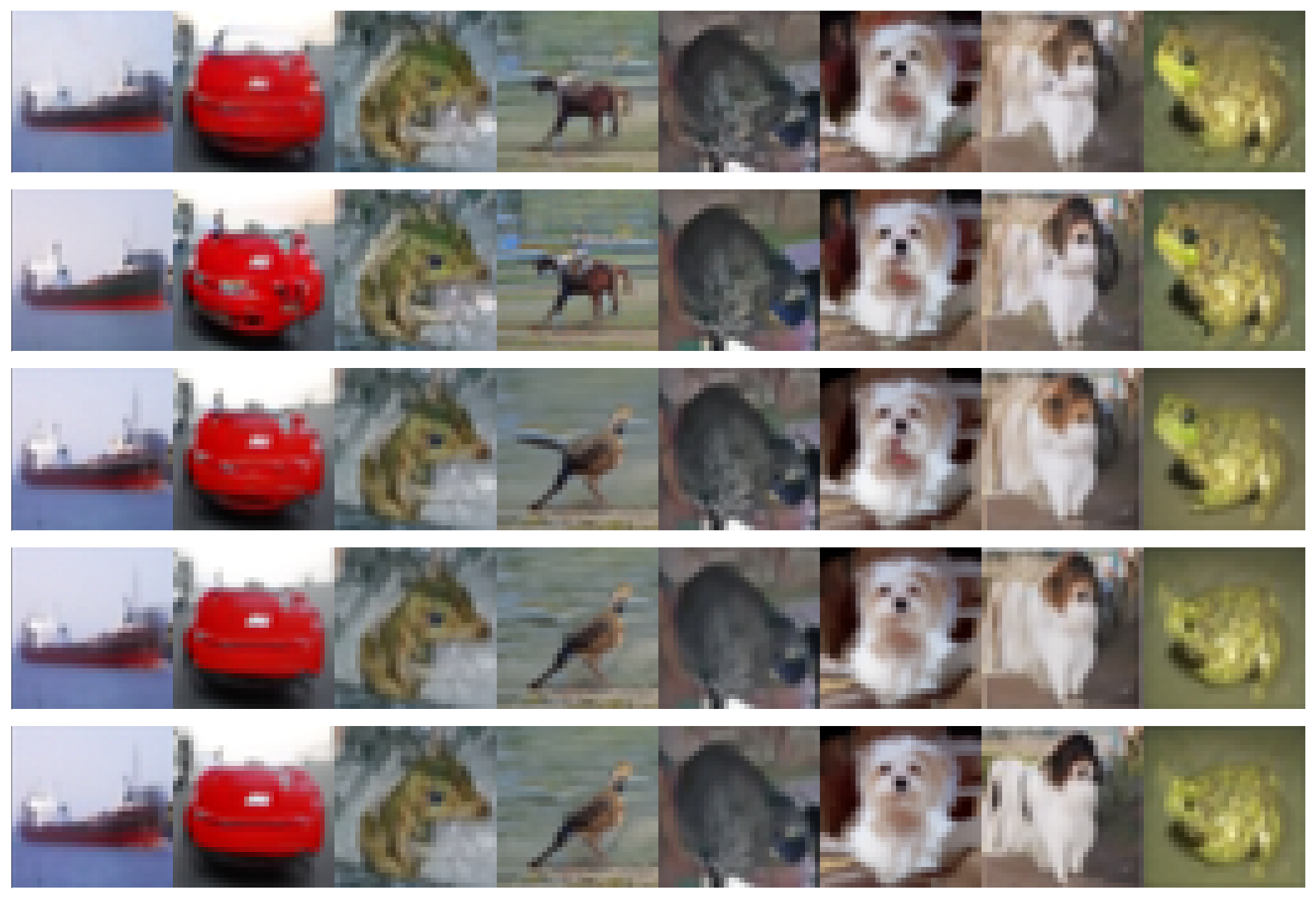
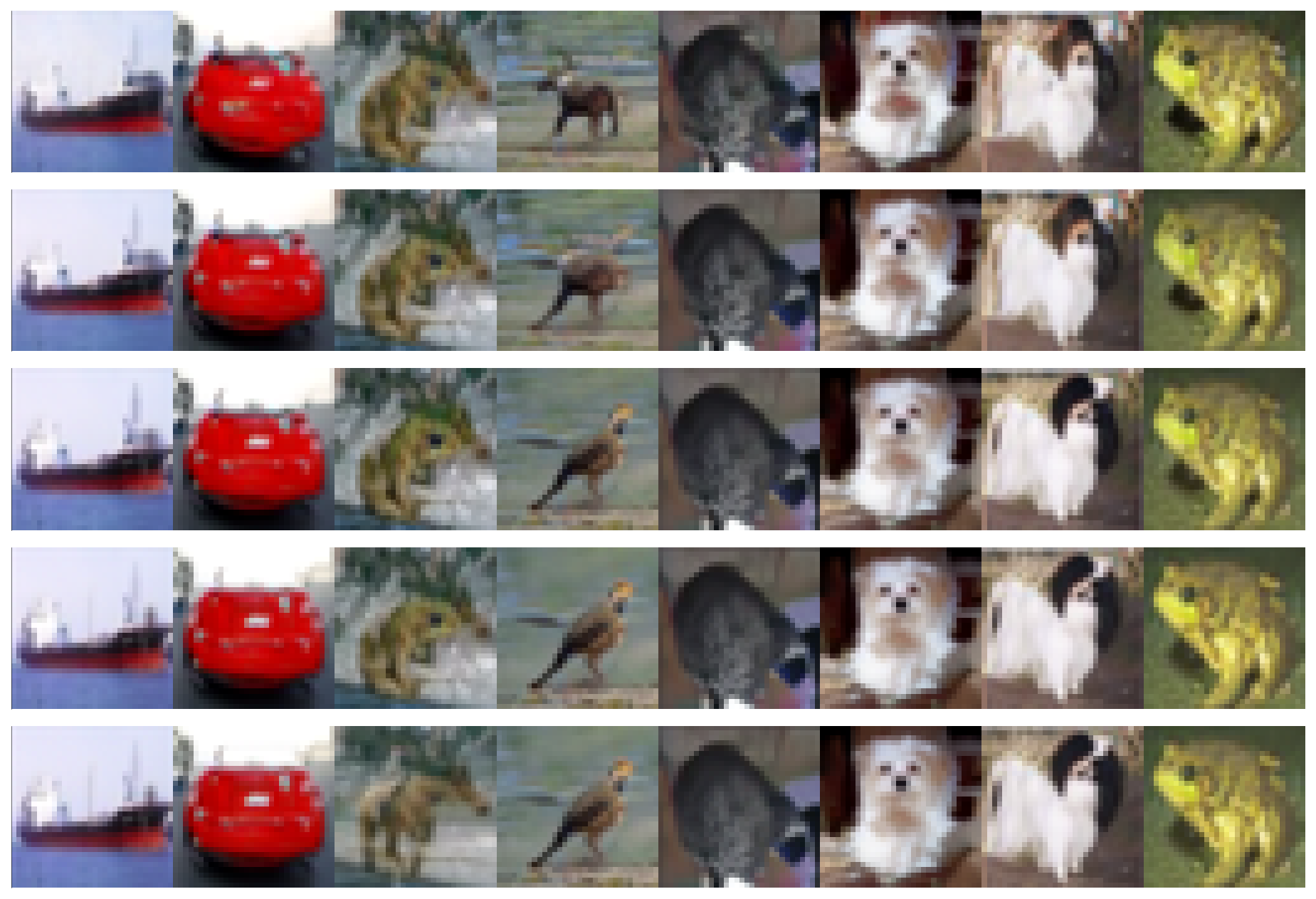
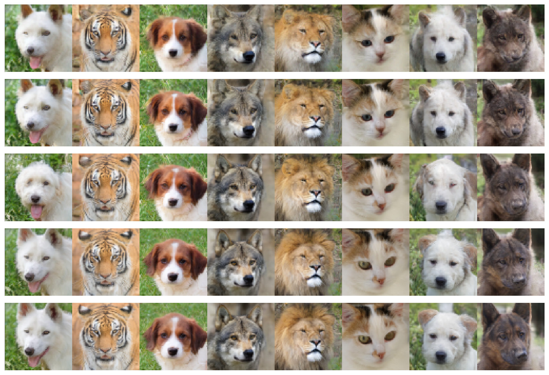
Qualitative Results. Progressive refinement comparison across methods, whereby we systematically increase the number of steps for a fixed random seed. All methods improve with more sampling steps. LSD produces higher quality samples at every step count compared to PSD variants. Each row shows samples at $N \in \{1, 2, 4, 8, 16\}$ steps from the same random seed.
CIFAR-10
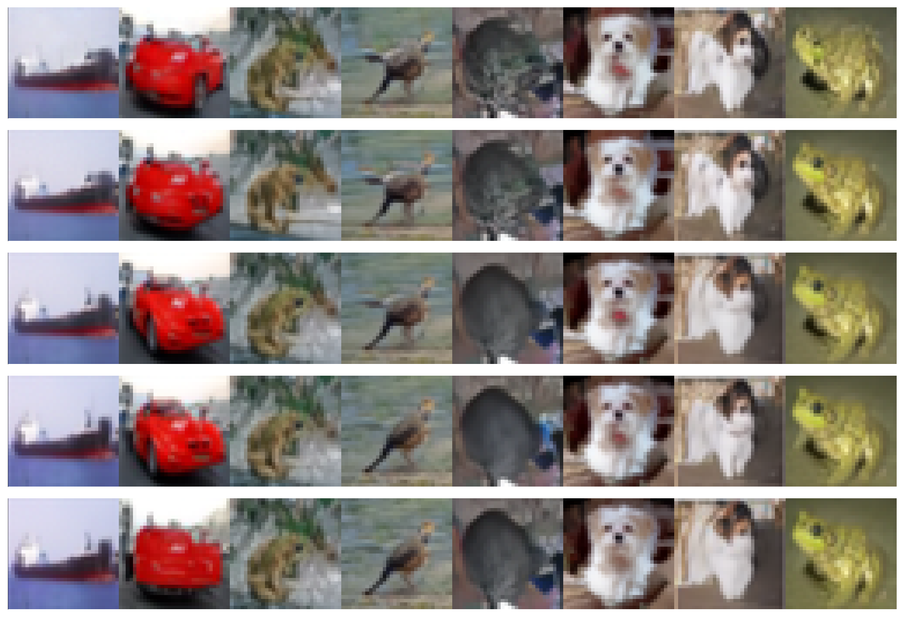
PSD-M
PSD-U
LSD
CelebA-64
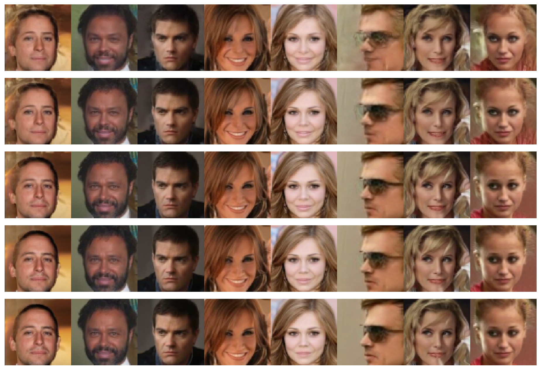
PSD-M
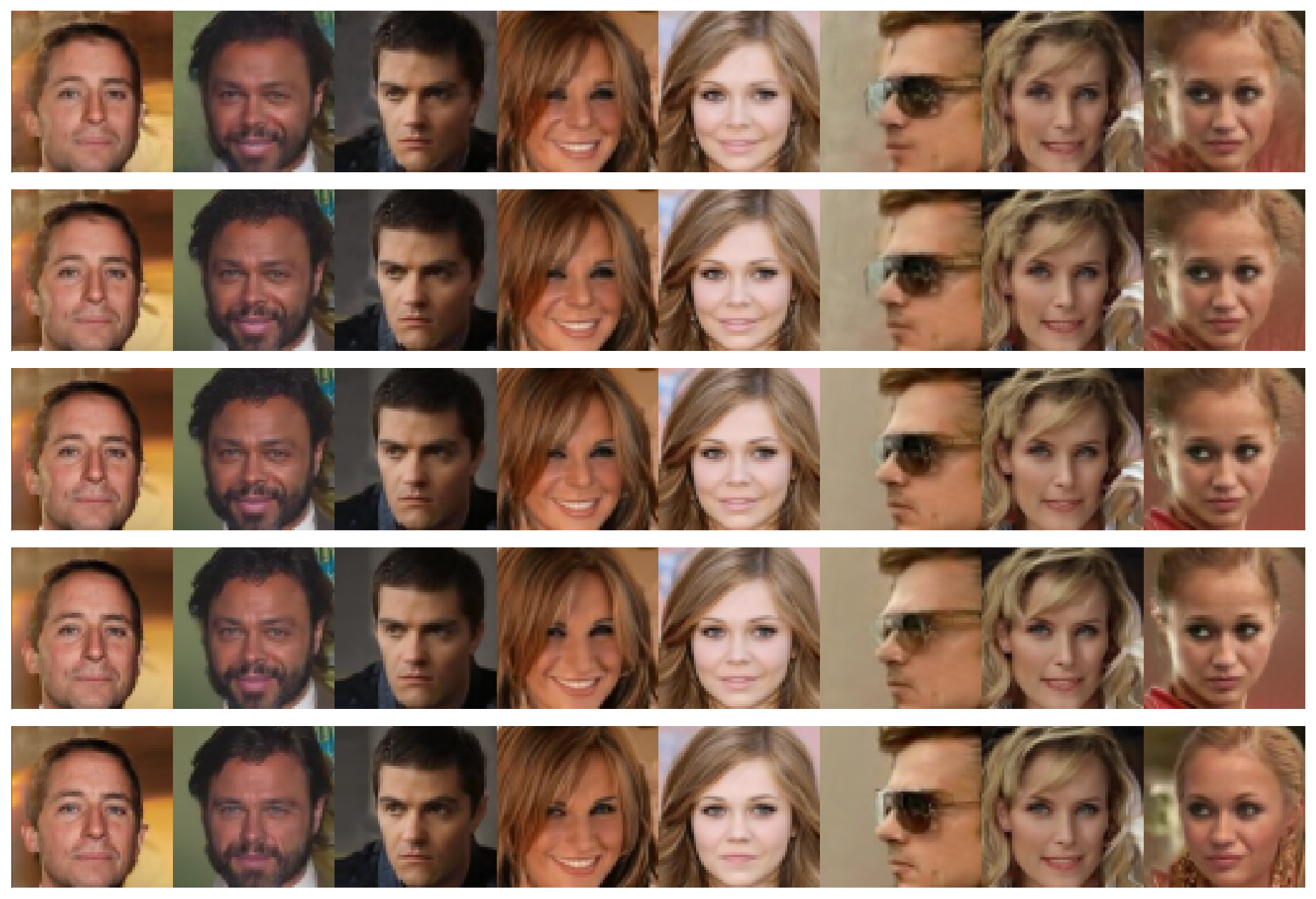
PSD-U
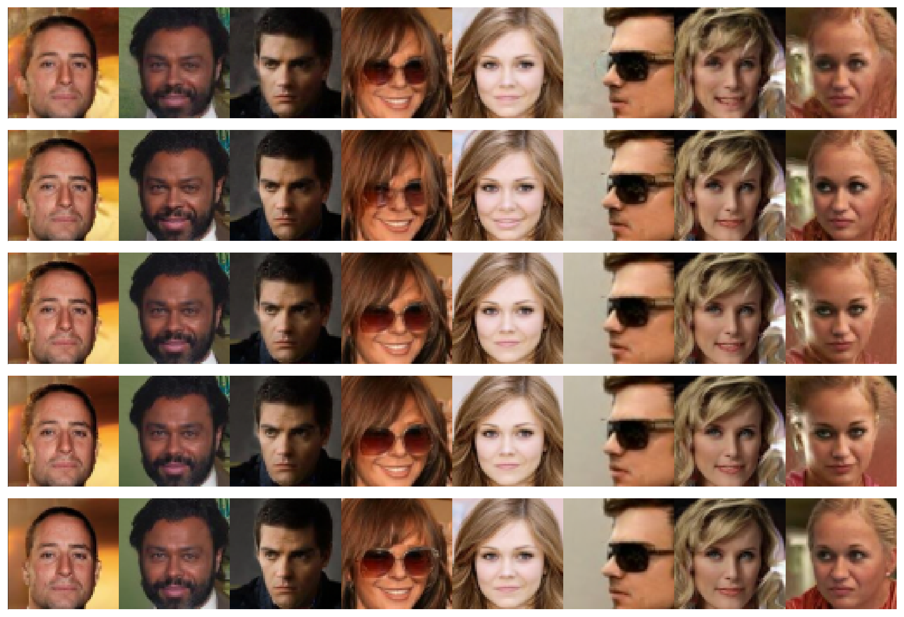
LSD
AFHQ-64
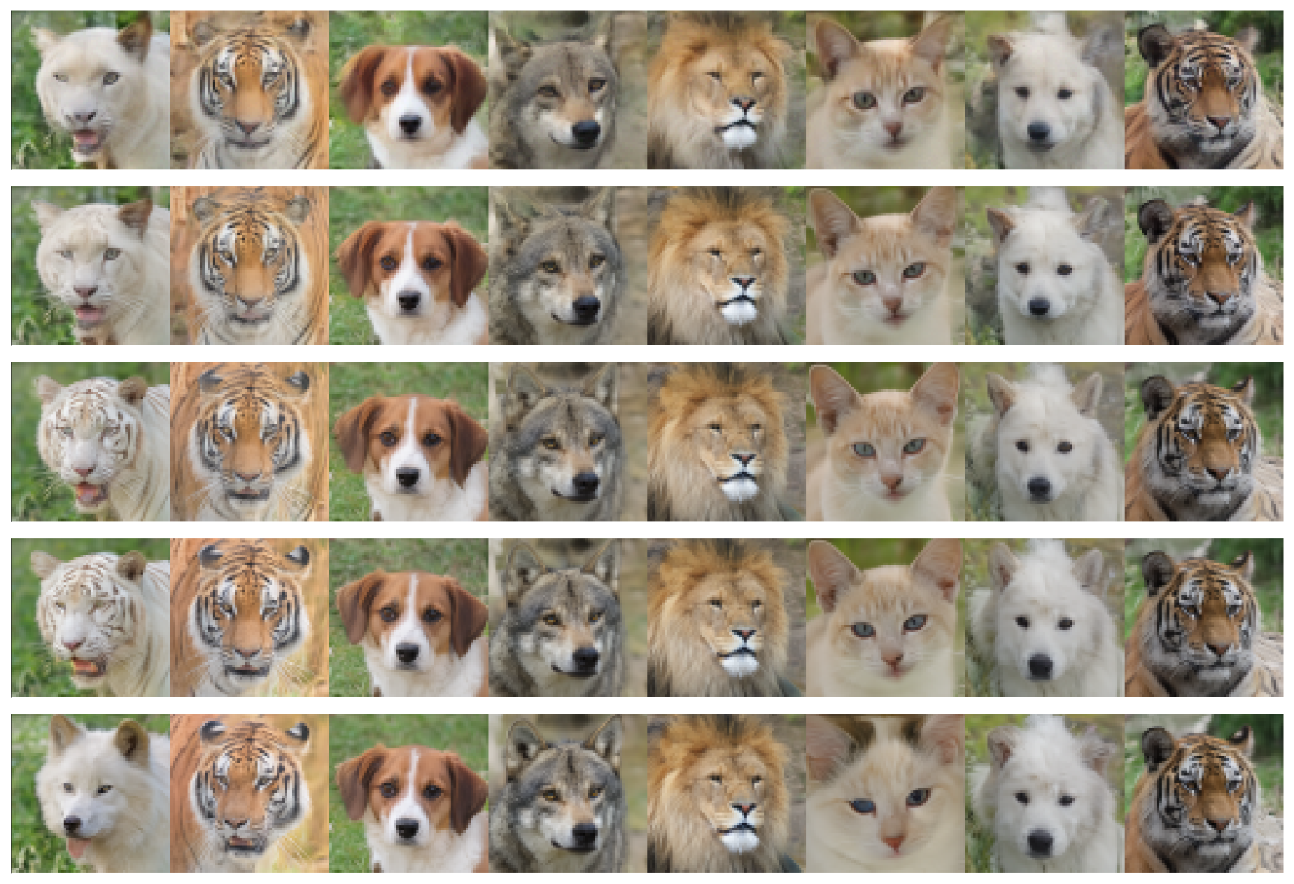
PSD-M
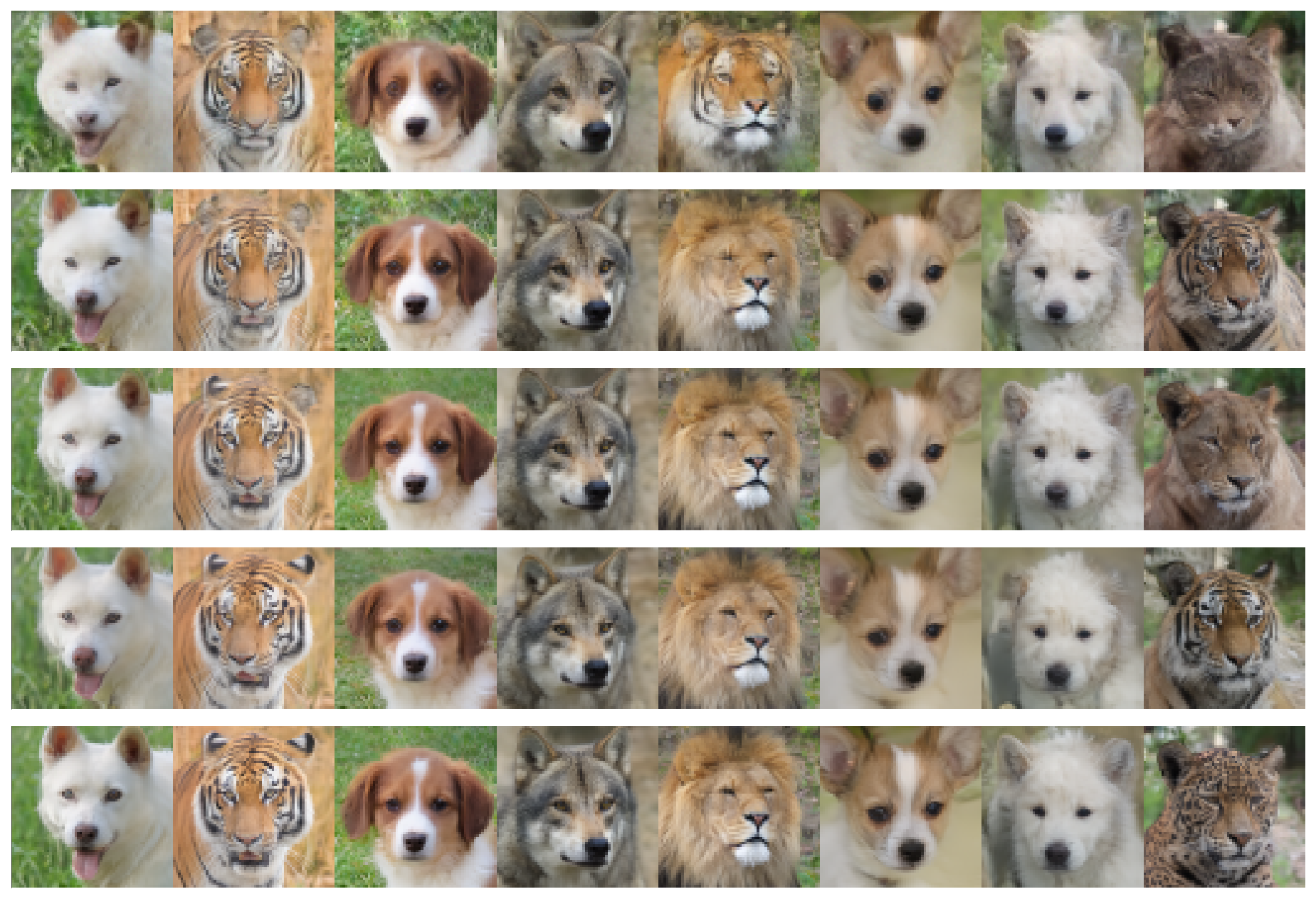
PSD-U
LSD
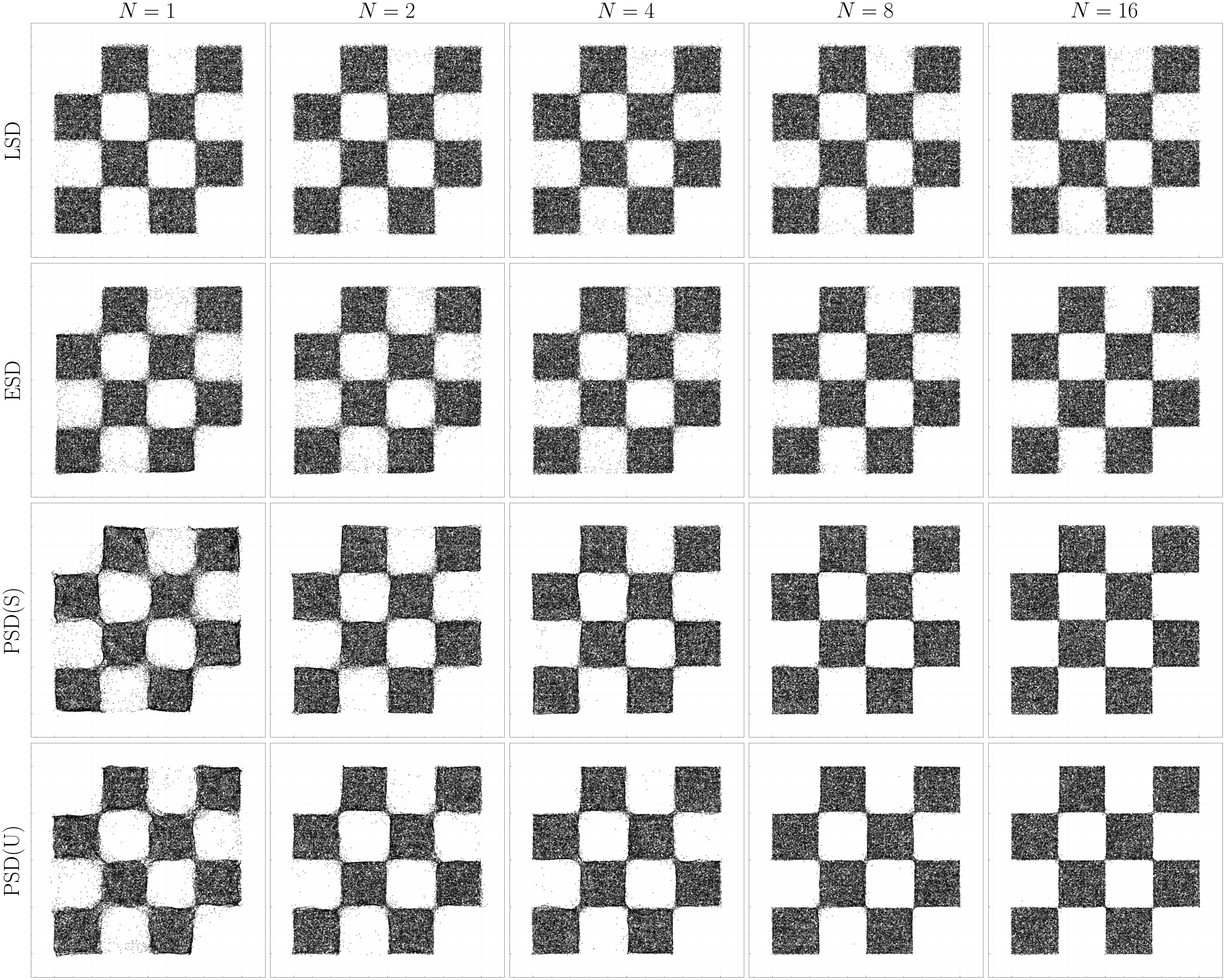
On the synthetic 2D checkerboard dataset -- a paradigmatic model of multimodality and sharp boundaries -- LSD captures the mode structure most accurately. Here, we found that ESD remained stable, likely due to the simpler network parameterization in this low-dimensional setting. ESD and PSD introduce artifacts or blur boundaries at low step counts. LSD achieves the best KL divergence across 1, 2, 4, and 8 steps.
| Method | 1 Step | 2 Steps | 4 Steps | 8 Steps | 16 Steps |
|---|---|---|---|---|---|
| LSD | 0.0864 | 0.0765 | 0.0708 | 0.0699 | 0.0710 |
| ESD | 0.0983 | 0.0921 | 0.0834 | 0.0816 | 0.0751 |
| PSD-M | 0.1456 | 0.0891 | 0.0812 | 0.0717 | 0.0689 |
| PSD-U | 0.1113 | 0.1067 | 0.0747 | 0.0727 | 0.0679 |
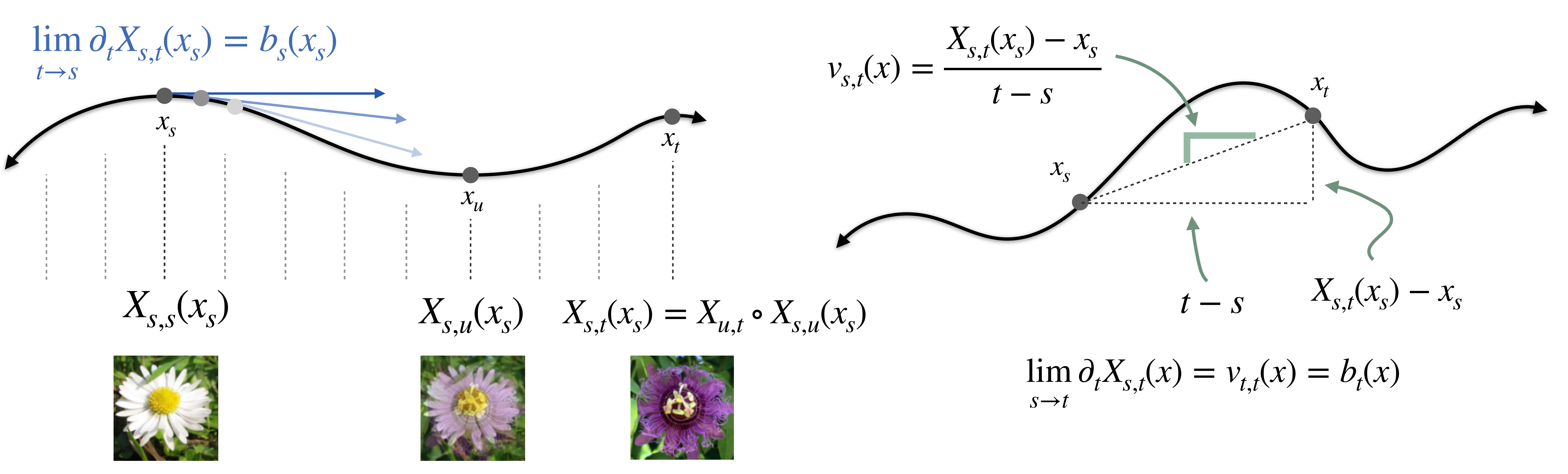
The flow map $X_{s,t}$ satisfies the defining property (or jump condition) that $X_{s,t}(x_s) = x_t$ for any trajectory $x_T$ of the probability flow $\dot{x}_t = b_t(x_t)$. One of our key insights is that the velocity field $b_t$ is implicitly encoded in the flow map itself:
Lemma (Tangent Condition): Let $X_{s,t}$ denote the flow map. Then, $$\lim_{s\to t}\partial_t X_{s,t}(x) = b_t(x) \quad \forall t \in [0,1], \; \forall x \in \mathbb{R}^d.$$
To exploit this algorithmically, we parameterize the flow map as $$X_{s,t}(x) = x + (t-s)v_{s,t}(x)$$ which automatically enforces the boundary condition $X_{s,s}(x) = x$. Taking the limit as $s \to t$: $$\lim_{s\to t}\partial_t X_{s,t}(x) = \lim_{s\to t}\partial_t[x + (t-s)v_{s,t}(x)] = v_{t,t}(x)$$ Combined with the tangent condition, we obtain the fundamental relation:
$$v_{t,t}(x) = b_t(x).$$
This shows that $v_{t,t}$ on the diagonal recovers the velocity field, which we can learn via standard flow matching. The challenge is then learning $v_{s,t}$ off the diagonal ($s \neq t$), which we address through self-distillation.
Given the parameterization $X_{s,t}(x) = x + (t-s)v_{s,t}(x)$ and the tangent condition $v_{t,t}(x) = b_t(x)$, we can characterize the flow map through three equivalent conditions:
Proposition (Flow Map Characterizations): Assume $X_{s,t}(x) = x + (t-s)v_{s,t}(x)$ with $v_{t,t}(x) = b_t(x)$.
Then $X_{s,t}$ is the flow map if and only if any of the following holds:
(i) Lagrangian condition:
$$\partial_t X_{s,t}(x) = v_{t,t}(X_{s,t}(x)) \quad \forall (s,t,x) \in [0,1]^2 \times \mathbb{R}^d$$
(ii) Eulerian condition:
$$\partial_s X_{s,t}(x) + \nabla X_{s,t}(x)v_{s,s}(x) = 0 \quad \forall (s,t,x) \in [0,1]^2 \times \mathbb{R}^d$$
(iii) Semigroup condition:
$$X_{u,t}(X_{s,u}(x)) = X_{s,t}(x) \quad \forall (s,u,t,x) \in [0,1]^3 \times \mathbb{R}^d$$
Each condition provides a different perspective on the flow map. The Lagrangian follows trajectories forward in time, the Eulerian describes transport via a partial differential equation, and the semigroup expresses composition of jumps. These yield three distinct self-distillation algorithms, as we now discuss.
Proposition (Self-Distillation): The flow map $X_{s,t}$ is given by $X_{s,t}(x) = x + (t-s)v_{s,t}(x)$
where $v_{s,t}$ is the unique minimizer of
$$\mathcal{L}(\hat{v}) = \mathcal{L}_b(\hat{v}) + \mathcal{L}_{\text{dist}}(\hat{v})$$
Here $\mathcal{L}_b$ is the flow matching loss on the diagonal:
$$\mathcal{L}_b(\hat{v}) = \int_0^1 \mathbb{E}_{x_0,x_1}\left[|\hat{v}_{t,t}(I_t) - \dot{I}_t|^2\right]dt$$
and $\mathcal{L}_{\text{dist}}$ is any of the following three distillation losses:
Lagrangian Self-Distillation (LSD):
$$\mathcal{L}_{\text{LSD}}(\hat{v}) = \int_0^1\int_0^t \mathbb{E}_{x_0,x_1}\left[\left|\partial_t \hat{X}_{s,t}(I_s) - \hat{v}_{t,t}(\hat{X}_{s,t}(I_s))\right|^2\right]ds\,dt$$
Eulerian Self-Distillation (ESD):
$$\mathcal{L}_{\text{ESD}}(\hat{v}) = \int_0^1\int_0^t \mathbb{E}_{x_0,x_1}\left[\left|\partial_s \hat{X}_{s,t}(I_s) + \nabla \hat{X}_{s,t}(I_s)\hat{v}_{s,s}(I_s)\right|^2\right]ds\,dt$$
Progressive Self-Distillation (PSD):
$$\mathcal{L}_{\text{PSD}}(\hat{v}) = \int_0^1\int_0^t\int_s^t \mathbb{E}_{x_0,x_1}\left[\left|\hat{X}_{s,t}(I_s) - \hat{X}_{u,t}(\hat{X}_{s,u}(I_s))\right|^2\right]du\,ds\,dt$$
By converting each characterization above into a training objective, we obtain three self-distillation algorithms that eliminate the need for pre-trained teachers while maintaining the stability of distillation.
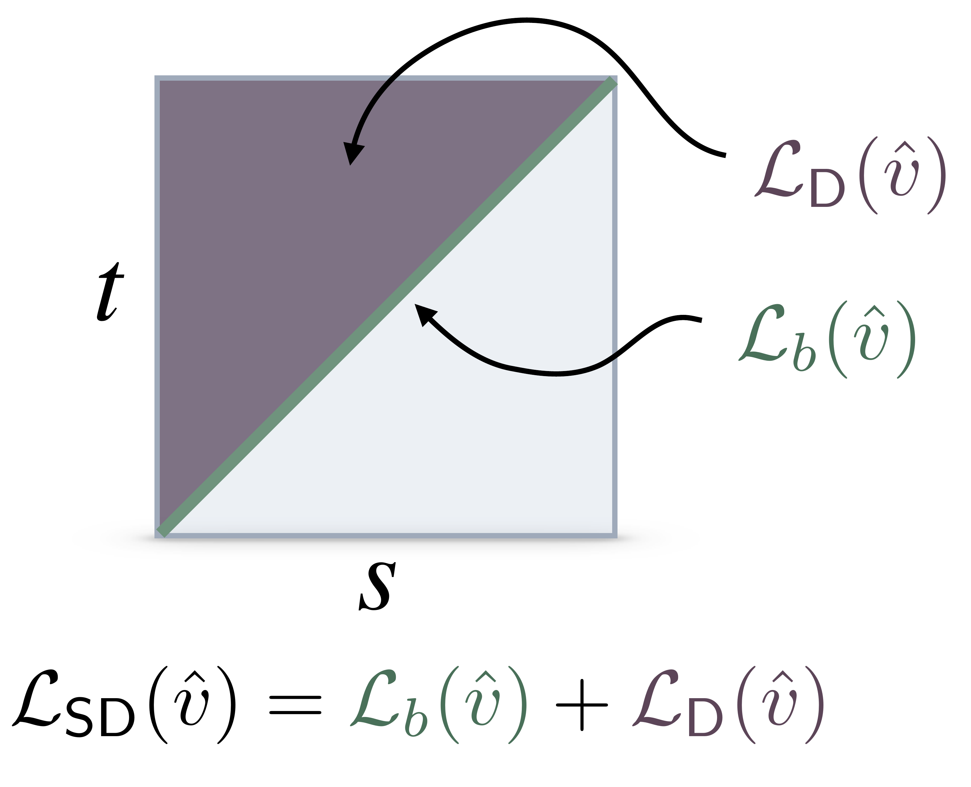
Our plug-and-play approach pairs any distillation objective on the off-diagonal $s \neq t$ with flow matching on the diagonal $s=t$.
In practice, it is useful to control the flow of information from the diagonal ($s=t$) to the off-diagonal ($s \neq t$). We can implement this with the stopgradient operator $\text{sg}(\cdot)$, which treats its argument as constant during backpropagation. This prevents gradient flow through specific terms, enabling us to simulate the setting where we have a pre-trained teacher. It is particularly important to avoid backpropagating through the spatial gradient $\nabla \hat{X}_{s,t}$ in the Eulerian loss, which is often numerically unstable and requires increased memory.
The practical losses we recommend with stopgradient are:
Lagrangian Self-Distillation (LSD):
Eulerian Self-Distillation (ESD):
Progressive Self-Distillation (PSD):
Recovering Known Methods: We show in the appendix of our paper that all known algorithms for training consistency models (including consistency training, consistency distillation, shortcut models, align your flow, and mean flow) can be recovered via an appropriate choice of stopgradient placement in our framework.
@misc{boffi2025buildconsistencymodellearning,
  title={How to build a consistency model: Learning flow maps via self-distillation},
  author={Nicholas M. Boffi and Michael S. Albergo and Eric Vanden-Eijnden},
  year={2025},
  eprint={2505.18825},
  archivePrefix={arXiv},
  primaryClass={cs.LG},
  url={https://arxiv.org/abs/2505.18825},
}

@misc{boffi2025flowmapmatchingstochastic,
  title={Flow map matching with stochastic interpolants: A mathematical framework for consistency models},
  author={Nicholas M. Boffi and Michael S. Albergo and Eric Vanden-Eijnden},
  year={2025},
  eprint={2406.07507},
  archivePrefix={arXiv},
  primaryClass={cs.LG},
  url={https://arxiv.org/abs/2406.07507},
}